Implementing Matrix-Tree Theorem in PyTorch
Melbourne,If you’re working on non-projective graph-based parsing, you may encounter a problem where you want to compute a quantity which can be factored into a sum over (non-projective) trees. One such quantity is the partition function of a CRF over trees. You realise that this isn’t straightforward because the number of trees can be exponential, so iterating over the trees isn’t going to work. You look for solutions in the literature, and you find something called Matrix-Tree Theorem (MTT), which provides an efficient way to compute the quantity. With MTT, this computation becomes as simple as taking the determinant of a matrix! Happily, you start trying to implement MTT. But it turns out MTT isn’t that obvious to implement. You’re struggling with two problems: (1) batching the computation, where each batch contains sentences of different lengths, and (2) ensuring numerical safety in the presence of very large arc scores.
That story is actually me when I was implementing MTT in PyTorch for our EACL work. In this article, I’d like to share my solutions to those problems, something that I wasn’t able to put on the paper. I’m going to start by giving some background on graph-based dependency parsing as well as the MTT itself in a bit more detail. Feel free to skip if you’re already familiar with them. Next, I explain the problem with batching the MTT computation and the solution I came up with. This is then followed by the issue of numerical safety, which is especially important with neural parsing, and a simple trick I used to deal with it, inspired by a similar trick in the safe computation of log-sum-exp.
Graph-Based Dependency Parsing
In graph-based dependency parsing, the parsing problem is cast as a search for the maximum spanning tree. Here, I’ll reproduce the formulation given by McDonald et al. (2005). Let \(\boldsymbol{x}=x_1\cdots x_n\) denote an input sentence, \(\boldsymbol{y}\) denote a dependency tree, and \(A(\boldsymbol{y})\) denote the set of arcs in \(\boldsymbol{y}\). So, we write \((h,m)\in A(\boldsymbol{y})\) if there is a dependency arc from \(x_h\) to \(x_m\). We say that the word \(x_h\) is the head of the word \(x_m\). A common formulation is to define the score of a tree as the sum of the scores of its arcs. Thus, the score of tree \(\boldsymbol{y}\) for sentence \(\boldsymbol{x}\) can be written as
where \(s(h,m,\boldsymbol{x})\) denotes the score of arc \((h,m)\) for \(\boldsymbol{x}\). In neural parsing, the arc scoring function \(s(h,m,\boldsymbol{x})\) is parameterised by a neural network. For each sentence \(\boldsymbol{x}\), we can define a directed graph \(G_\boldsymbol{x}=(V_\boldsymbol{x},E_\boldsymbol{x})\) where
is the set of vertices with \(x_0\) being the root node, and
is the set of edges. For example, if \(\boldsymbol{x}=x_1x_2\) then \(V=\{x_0=\text{ROOT},x_1,x_2\}\) and \(E=\{(0,1),(0,2),(1,2),(2,1)\}\) (subscripts are dropped hereinafter for brevity). Dependency trees for \(\boldsymbol{x}\) and spanning trees of \(G\) (rooted at \(x_0\)) coincide, so finding the highest scoring dependency tree for \(\boldsymbol{x}\) is equivalent to finding the maximum spanning tree in \(G\). A property that will be important later is that all spanning trees of \(G\) have exactly \(n\) arcs. In code, \(G\) can be represented by a score matrix \(\mathbf{S}\in\mathbb{R}^{(n+1)\times(n+1)}\) where \(S_{hm}=s(h,m,\boldsymbol{x})\). It is common to define a CRF over dependency trees:
where
is called the partition function and \(\mathcal{Y}(\boldsymbol{x})\) is the set of all possible dependency trees for \(\boldsymbol{x}\) (rooted at \(x_0\)). Computing this partition function efficiently can be a challenge as there is an exponentially large number of trees in \(\mathcal{Y}(\boldsymbol{x})\).
Matrix-Tree Theorem
Matrix-Tree Theorem (MTT) allows an efficient computation of the partition function. First, we represent \(G\) in a weight matrix \(\mathbf{W}\in\mathbb{R}^{(n+1)\times(n+1)}\) where \(W_{hm}=\exp S_{hm}\). Observe that
Next, we define the Laplacian matrix \(\mathbf{L}\in\mathbb{R}^{(n+1)\times(n+1)}\) for \(\mathbf{W}\) where
and let \(\mathbf{L}^{(k)}\) denote the matrix \(\mathbf{L}\) with its row and column \(k\) removed. MTT states that
In other words, computing the huge sum in \(Z(\boldsymbol{x})\) can be done as efficiently as taking a determinant of a matrix, which runs in polynomial time! With PyTorch, MTT can be written as simply as:
from torch import LongTensor, Tensor
import torch

def mtt(scores: Tensor) -> Tensor:
    """Run MTT on the graph represented by the given scores.

    Args:
        scores: Tensor of shape (B, N, N) containing score of all possible arcs.

    Returns:
        1-D tensor of length B, each is the MTT result for a sentence in the batch.
    """
    bsz, slen, slen_ = scores.shape
    assert slen == slen_, "scores.size(1) and scores.size(2) must be equal"
    weights = scores.exp()

    laplacian = -weights
    # Zero out entries in the main diagonal
    laplacian.masked_fill_(torch.eye(slen).bool(), 0)
    w = weights.masked_fill(torch.eye(slen).bool(), 0)
    # Fill the main diagonal with the correct value
    laplacian += torch.diag_embed(w.sum(dim=1))

    # Compute log partition function with MTT
    log_partition = laplacian[:, 1:, 1:].logdet()
    assert log_partition.shape == (bsz,)
    return log_partition
We compute the log determinant because it’s more numerically safe for large matrices. Here, we assume unlabelled parsing and allow the root node to have more than one child for simplicity. In some treebank, the root node may be constrained to have exactly one child. Also, MTT can be used to compute arc marginal probabilities efficiently, which we won’t explain here. All these cases can be handled quite easily (Koo et al., 2007).
Batching MTT Computation
Batching computation over multiple sentences with different lengths means that there are sentences padded with padding tokens. Arcs incident to these padding tokens can make the partition function wrong because they make the MTT computation counts invalid trees. The figure below illustrates the problem when there is a single word and a single padding token in a sentence.
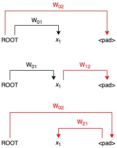
Three possible spanning trees with invalid arcs incident to the padding token in red.
The figure shows all three possible spanning trees for the input sentence. Note that there is actually just a single valid tree (in black), but the presence of the padding token <pad> makes as if there are three. Thus, if we compute the partition function of the graph, we will get \(W_{01}W_{02}+W_{01}W_{12}+W_{02}W_{21}\), whereas the correct result is just \(W_{01}\).
To solve the problem, we must ensure that we only count each valid tree once, and the arcs incident to the padding tokens don’t contribute to the partition function. To do so, we can force padding tokens to always have the root token as the head and ensure that the corresponding arcs have a weight of one. Furthermore, any other arcs incident to the padding tokens must have zero weight. This can be achieved by defining a new weight matrix \(\mathbf{W}'\) where
and then running MTT with the new weight matrix \(\mathbf{W}'\). The result will be the same as running MTT with no padding tokens. In PyTorch, the above can be implemented as follows:
# `is_pad` is a boolean tensor indicating which tokens are padding
assert is_pad.shape == (bsz, slen)
incident_to_pad = is_pad.unsqueeze(1) | is_pad.unsqueeze(2)
assert incident_to_pad.shape == (bsz, slen, slen)
# Set scores of arcs incident to padding tokens to a large negative number
# so they become very close to zero after exp
scores.masked_fill_(incident_to_pad, -1e9)
# Set scores of arcs from the root to padding tokens to zero so they become one
# after exp
scores[:, 0].masked_fill_(is_pad, 0.)
Continuing the illustration above, the above steps mean setting \(W'_{12}=W'_{21}=0\), \(W'_{02}=1\), and keep the other weights unchanged. That is, we set the weight of the arc from \(x_1\) to <pad> and from <pad> to \(x_1\) to zero, and of the arc from the root to <pad> to one. As a result, the partition function becomes
as desired.
Making MTT Numerically Safe
To obtain the positive arc weights, we take the exp of the arc scores, as is customary when working with deep learning. However, the result of exp may overflow if the input is sufficiently large [1]. This can happen in the context of neural parsing as the arc scores come from a neural network and thus are unbounded. When the exp result overflows, so will the partition function, rendering it meaningless.
A solution to this problem is simple: subtract the maximum arc score from all the arc scores before taking the exp.
max_score, _ = scores.reshape(bsz, -1).max(dim=1)
assert max_score.shape == (bsz,)
weights = (scores - max_score.reshape(bsz, 1, 1)).exp()
assert weights.shape == scores.shape
This basically shifts the scores lower so that the largest arc scores become zero, which won’t overflow for exp, and smaller arc scores become negative, which won’t either. Once the subtraction is done, we can safely take the exp to get the arc weights, and MTT can proceed as usual. However, we must be careful when computing the maximum arc score not to include scores from invalid tree arcs, which are arcs incident to the padding tokens, incoming to the root, and self-loops. We must set the scores of these arcs to a large negative number before computing the maximum arc score so they’ll be ignored by the max operation. We already did so for arcs incident to the padding tokens when we batch MTT. Thus, we only need to take care of arcs incoming to the root and self-loops.
# Set scores of arcs incoming to root
scores[:, :, 0] = -1e9
# Set scores of self-loops
scores.masked_fill_(torch.eye(slen).bool(), -1e9)

### Subtraction and exp go here ###
Additionally, we must ensure that the weights from the root node to the padding tokens are still equal to one even after the subtraction so our trick to batch MTT still works properly. This can be achieved by setting the weights directly instead of the scores.
# The line below is commented out/not needed because now we set the
# arc weights directly after taking the exp
#scores[:, 0].masked_fill_(is_pad, 0.)

### Subtraction and exp go here ###

weights[:, 0].masked_fill_(is_pad, 1.)
We’re almost finished. One last issue: if the scores are very negative after the subtraction, taking the exp will result in zero arc weights because they underflow. These zero arc weights are problematic because the weight of the tree containing any of those arcs will also be zero. To remedy this issue, we can add a small positive value to the arc weights, preventing them from being exaclty zero, before proceeding with MTT.
# Add small positive value after exp
weights = (scores - max_score.reshape(bsz, 1, 1)).exp() + 1e-8
assert weights.shape == scores.shape
We’re almost there! The very last thing to note is that, at the end, we must correct the result by adding the maximum score back, multiplied by \(n\) which is the number of arcs in the spanning tree.
# `length` is a 1-D tensor giving the lengths of each sentence
# (including ROOT) in the batch
assert length.shape == (bsz,)
log_partition = log_partition + (length.float() - 1) * max_score
And we’re done! The key idea behing this trick is: subtracting any constant from all the arc scores is equivalent to dividing all the weights by the exp of that constant, which can then be factored out from the sum. Formally,
for any \(c\neq0\) where the last step is possible because \(|A(\boldsymbol{y})|=n\) for all \(\boldsymbol{y}\), i.e. all spanning trees of \(\boldsymbol{x}\) has the same number of arcs, which is \(n\). A similar trick is also used for numerically safe computation of log-sum-exp.
Putting It All Together
The complete PyTorch code is given below:
from typing import Optional
from torch import LongTensor, Tensor
import torch

def log_partition(scores: Tensor, length: Optional[LongTensor] = None) -> Tensor:
    """Compute log partition function over dependency trees with MTT.

    Args:
        scores: Tensor of shape (B, N, N) containing score of all possible arcs.
        length: 1-D tensor of length B giving the lengths of sequences in the batch.

    Returns:
        1-D tensor of length B containing the log partition function.
    """
    bsz, slen, slen_ = scores.shape
    assert slen == slen_, "scores.size(1) and scores.size(2) must be equal"
    if length is None:
        length = torch.full([bsz], slen).long()
    else:
        assert length.shape == (bsz,), f"length must be a 1-D tensor of length {bsz}"

    is_pad = torch.arange(slen) >= length.unsqueeze(1)
    assert is_pad.shape == (bsz, slen)
    incident_to_pad = is_pad.unsqueeze(1) | is_pad.unsqueeze(2)
    assert incident_to_pad.shape == (bsz, slen, slen)

    # Set scores of arcs incident to padding tokens, incoming to root,
    # and self-loops to a large negative number so they become very close
    # to zero after exp and are also ignored by the max operation below
    scores.masked_fill_(incident_to_pad, -1e9)
    scores[:, :, 0] = -1e9
    scores.masked_fill_(torch.eye(slen).bool(), -1e9)

    # Shift scores to lie in safe range for exp
    max_score, _ = scores.reshape(bsz, -1).max(dim=1)
    assert max_score.shape == (bsz,)
    weights = (scores - max_score.reshape(bsz, 1, 1)).exp() + 1e-8
    assert weights.shape == scores.shape

    # Set weights of arcs from the root to padding tokens to one
    weights[:, 0].masked_fill_(is_pad, 1.)

    # Create Laplacian matrix
    laplacian = -weights
    # Zero out entries in the main diagonal
    laplacian.masked_fill_(torch.eye(slen).bool(), 0)
    w = weights.masked_fill(torch.eye(slen).bool(), 0)
    # Fill the main diagonal with the correct value
    laplacian += torch.diag_embed(w.sum(dim=1))

    # Compute log partition function with MTT
    log_partition = laplacian[:, 1:, 1:].logdet()
    assert log_partition.shape == (bsz,)

    # Correct result
    log_partition = log_partition + (length.float() - 1) * max_score

    return log_partition
The code above may need to be modified slightly if e.g., your tensors are on CUDA devices, but it basically works. There are other variants of MTT, for example one that sums over single-rooted trees, which isn’t explained here. The paper by Koo et al. (2007) explains all these variants clearly, and the code above can be adopted to them with minimal modifications. The code for our EACL work implements all of these variants (with a slightly different style from the code presented here) so you can just use it right away if you want.
| [1] | In PyTorch 1.6.0, the threshold seems to be around 88.7. Anything larger than that results in inf when fed into torch.exp. |